Hypothesis Testing

Introduction

• Testing hypothesis is an essential part of statistical inference
• A statistical hypothesis is an assumption about a population. This assumption may or may not be true.
• For example, claiming that a new drug is better than the current drug for treatment of the same symptoms.
• The best way to determine whether a statistical hypothesis is true would be to examine the entire population.
• Since that is often impractical, researchers typically examine a random sample from the population. If sample data are consistent with the statistical hypothesis, the hypothesis is accepted; if not, it is rejected.

There are two types of statistical hypotheses

• Null Hypothesis

• The null hypothesis denoted by H0, is usually the hypothesis that sample observations result purely from chance. 
• H0:=
• H1:≠ : two-tail test
• H1:</> : one-tail test

• Alternative Hypothesis 

• The alternative hypothesis, denoted by H1 is the hypothesis that sample observations are influenced by some non-random cause.
• H1 or Ha
• For example, suppose we wanted to determine whether a tossing a coin was fair and balanced, A null hypothesis might be that half the flips would result in heads and half in tails. The alternative hypothesis might be that the number of heads and tails would be very different. symbolically there hypotheses would be expressed as
• H0:P = 0.5
• Ha:P ≠ 0.5
• Statisticians follow a formal process to determine whether to accept or reject a null hypothesis, based on sample data. This process called hypothesis testing, consists of five steps
1. State Null and alternative hypothesis (based on population mean.)
2. Write down relevant data, select a level of significance;α (rejection area)
3. Identify and compute the test statistic Z to be used in testing the hypothesis.
4. Compute the Critical values(the line which is between rejection area and non rejection area) (boundary) Zc
5. Based on the sample arrive a decision

Use the following formula for test statistic/Z value as follows

• if the standard diviation is  known
• number of sample>30

Remember this formula is for Testing Hypotheses about Single Means when the poplation Variance is known.
But when the population variance is unknown, we must use the standard deviation s, to estimate σ
We use t distribution instead of Z distribution.

• if the standard deviation is unknown
• number of sample < 30

Decision Errors

• Two types of errors can result from a hypothesis test.
• Type I error: A type I error occurs when the null hypothesis is rejected when it is true. Type I error is called the significance level. This probability is also denoted by alpha, α.
• Type II error: A type II error occurs when the researcher accepts a null hypothesis that is false. H0 is accepted. 

Null Hypothesis	Accept H0	Reject H0
H0 isTRUE	Correct Decision	Type I error
H0 is FALSE	Type II error	Correct Decision

One-Tailed Tests

• A test of a statistical hypothesis where the region of rejection is on only one side of the sampling distribution, is called a one tailed test.
• For example suppose the null hypothesis states that the mean is equal to or more than 10. The alternative hypothesis would be that the mean is LESS than 10.
• The region of rejection would consist of a range of numbers located on the LEFT side of sampling distribution, that is a set of numbers LESS than 10.

Two-Tailed Tests 

• A test of a statistical hypothesis, where the region of rejection is on both sides of the sampling distribution, is called a two-tailed test.
• For example, suppose the null hypothesis states that the mean is equal to 10. The alternative hypothesis would be that the mean is less than 10 or greater than 10.
• The region of rejection would consist of a range of numbers located on both sides of sampling distribution; that is the region of rejection would consist party of numbers that were less than 10 and partly of numbers that were greater than 10.

df=degree of freedom =n-1

The concept

• The concept of degrees of freedom is central to the principle of estimating statistics of populations from samples of them
• The number of scores that are free to vary
• In many situations, the degrees of freedom are equal to the number of observations minus one.
• Used if the sample number is LESS than 30.

Confidence Interval for a population proportion

95% and 99% Confidence Intervals for µ

• The 95% and 99% Confidence Intervals for µ are constructed as follows when n>30 
• 95% CI for the population mean is  given by 
  
• 99% CI for the population mean is given by
  
• In general a confidence interval for the population mean is computed by
  

Standard Error of the Sample Means

• The standard error of the sample means is the standard deviation of the sampling distribution of the sample means.
• it is computed by 

General Concepts of Estimation

Point estimate

A point estimate is one value ( a point) that is used to estimate a population parameter.

Examples of point estimates are the sample mean, the sample standard deviation, the sample variance, the sample proportion etc...

EXAMPLE: The number of defective items produces by a machine was recorded for five randomly selected hours during a 40-hour work week, The observed number of defectives were 12, 4, 7, 14 and 10. So the sample mean is 9.4  thus a point estimate for hourly mean number of defectives is 9.4.

 Interval Estimate

• An Interval Estimate states the range within a population parameter probably lies. 
• The  interval within a population parameter is expected to occur is called a confidence interval.
• The  two confidence intervals that are used extensively are the 95% and the 99%
• The confidence level describes the uncertainty associated with a sampling  method.
• Suppose we used the same sampling method to select different samples and to compute a different interval estimate for each sample. some interval estimates would include the true population parameter and some would not. A 90% confidence level means that we would expect 90% of the interval estimates to include the population parameter.
• A 95% confidence interval means 95% of the sample means for a specified sample size will lie within 1,96 standard deviations of the hypothesized population mean.
• For the 99% confidence interval, 99% of the sample means for a specified sample size will lie within 2.58 standard deviation of the hypothesized population mean.

Statistical Inference

• Statistical inference refers to the use of information obtained from a sample in order to make decisions about unknown quantities in the population of interest.
• Since all population may be characterized or fully described by their parameters, it is important to make inferences on the one or more parameters whose values are unknown
• There are two main types of inferences
1. The hypothesis testing branch involves making decisions concerning the value of a parameter by testing a per-conceived hypothesis.
2. The estimation branch involves estimating or predicting the unknown value of a parameter.
• Both approaches involves the use of sample information in the form of sample statistic corresponding to the population parameter in question.
• Both approaches also rely on the "goodness" of the inference, which requires complete knowledge of the sampling distribution.

Estimation

• Up to this point we have assumed that the parameters of the population of interest are unknown.
• When dealing with methods such as normal distribution, the population mean, µx and standard deviation σx were given.
•  In estimation, there is a complete change in the type of problem with which we are concerned.
• Now we have to get used to dealing with problems where the population parameter of interest is either completely unknown or is given as a hypothetical(assumption) value. Solving these problem involves statistical inference.
• The general concepts of estimation
  1. θ represent any parameter of interest. e.g. the parameter whose value is unknown and must be estimated.
  2. Ô sample statistic that will be used to estimate unknown θ. 
  3. σÔ represents the standard error sample statistic,Ô. This measures the variability or error associated with all possible values of Ô as an estimate of θ
• There are two possibilities of determining population parameters - we can either calculate it exactly or we can estimate it.

Empirical Rule

Applies to mound shaped and symmetric probability density.

• P (µ - σ < X <µ + σ) = 0.68 
• P (µ - 2σ < X <µ + 2σ) = 0.95 
• P (µ - 3σ < X <µ + 3σ) = 0.997

Random Variable

• A random variable represents a possible outcome (usually numeric) from a random experiments&amp
  • Let X be random variable for a number of heads in 3 coin flips 
  • X represents any value from sample space {0, 1, 2 or 3)
• An observation is a realization of random variable
  • Let x be an observed number of heads in 3 coin tosses, eg x = 0

Bernuolli Trials:

• Random trial with two outcomes. Eg. Success or Failure. 
• Random variable X often coded as 0 (Failure) and 1 (Success)
• Bernuolli Trail has probability of success usually denoted p. Eg. P (Success) = p (x =1) = p 
• Accordingly, probability of failure (1 – p) is usually denoted q = 1 - p. 
• Eg. p (Failure) = 1 – p = q 
• Probability of Bernuolli’s Distribution is: 
• Where x can be zero or one
• The Binomial Distribution which consists of a fixed number of statistically independent Bernoulli trials

Binomial Distributing Function:

Poisson Random Variable:

Poisson random variable represents the number of independent events that occur randomly over unit of times 

Example:

• Number of calls to a call centre in an hour 
• Number of floods in a river in a year 
• Number of misprint in a page

Characteristic:

• Count number of times as event occur during a given unit of measurement (e.g. time, area). 
• Number of events that occur in one unit is independent of other units. 
• Probability that events occurs over given unit is identical for all units (constant rate) 
• Events occur randomly 
• Expected number of events (rate) in each unit is denoted by λ (lambda)

Poisson Distribution:

• Let x be Poisson random variable for number of independent events over unit of measurements. 
• To define probability distribution need to know: rate of unit occurrence per unit - λ .

Probability

Notion of probability:

• An event is a particular result or set of results
• A possibility space is the set of all possible outcomes
• Fro equally likely outcomes, the probability of an event E is given by

Compound event probability:

"A measure of the likely-hood that a compound event will occur" Method of calculating compound event probability

• Formulas
  • Additive rule
  • Conditional probability formula
  • Multiplicative rule
• Venn Diagram and Tree Diagram

Additive rule:

Mutually exclusive events:

• Both events cannot occur at the same time
  • Both male and female for one person
  • Both heads and tails for one coin toss
• No sample points in common(overlap)
  • All female students who are Muslim in room 102
  • All male students who are Christian in class room 103

Therefore probability of mutually exclusive events happening together is 0

Example:

additive rules for mutually exclusive events:

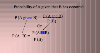
conditional probability

"probability of one event occurring given that another event has occurred"

Characteristics

• Restrict original sample space to account for new information
• Assumes probability of given event ≠ 0

Conditional probability:

P( B | A ) represents the probability of event B occurring given that event A has already occurred.
Suppose we draw two cards from a deck of 52.
Find the probability that the second card is a Jack given that the first card was a Jack and it was not replaced.
P( J2 | J1 ) = 3/51 ≈ 0.059
Find the probability that the second card is a Jack given that the first card was a Jack and it was replaced.
P( J2 | J1 ) = 4/52 = 1/13 ≈ 0.077

We can use the Multiplication Rule to calculate the probability of consecutive events.
 P( A and B ) = P(A) ∙ P( B | A )
 If events A and B are independent, then
P( A and B ) = P(A) ∙ P(B)

Conditional probability using Venn diagram:

Venn diagrams or set diagrams are diagrams that show all possible logical relations between a finite collection of sets (aggregation of things). Venn diagrams were conceived around 1880 by John Venn. They are used to teach elementary set theory, as well as illustrate simple set relationships in probability, logic, statistics, linguistics, and computer science.

Multiplicative rule: 

Independent events:

"The occurrence of one event does not influence the probability of another event"

To test for independence:

• P (A|B) = P (A)
• P (B|A) = P (B)
• P (A ∩ B) = P (A) * P (B)

Tree Diagram:

"A branched picture of multiplicative rule and used for finding (A ∩ B)”

Characteristics:

• Each set of branches is an event 
• Each set of branches should add up to 1 
• Multiply along each branch to find the probability of particular event

Example:
In a certain clothing shop, 40% of shoppers try on a jacket when browsing. Of those who try on jacket, 70% will subsequently purchase a jacket. However, 15% of browsers buy a jacket without trying on. What is the probability that a person who buys a jacket has tried one on?
Solution: Tree diagram
Let, Event (A) = customer tries on a jacket
       Event (B) = Customer buys a jacket First,
Find P(A) and then P(A|B)

Measures of Dispersion

Range:

The difference between the largest and the smallest numbers in the dataset.
The disadvantage of using range is that it does not measure the spread of the majority of valuses in a data set. It only measures the spread between highest and lowest values.

The Interquartile Range:

 The difference between the lower quartile and the upper quartile in the data set.

• Example:
• 87, 88, 88, 89, 90, 90, 90, 92, 93, 93, 95
• The Mean is the sixth value, 90
• Now consider the lower half of the data which is 87, 88, 88, 89, 90 and the middle of this set called lower quartile Q1 = 88
• The upper half of the set is 90, 92, 93, 93, 95 and the middle, called the upper quartile, Q3= is 93
• Therefore the interquartile is
• IQR = Q3 –Q1 =93 -88 = 5

Quartile Deviation:

half the distance between the third quartile, Q3, and the first quartile.
 QD = [Q3 - Q1]/2

Box Plots:

A graphical display based on quartiles that helps to picture a set of data.
Five pieces of data are needed to construct a box plot:

• The minimum Value
• The first quartile
• The median
• The third quartile
• The maximum value

Mean Deviation:

Another method for indicating the spread of results in data set.
Determine the average mean and the average value of the deviation of each score from the mean.
Thus each data point is taken into account
The average of the absolute values of the deviations from mean

Steps

• Find the mean or median or mode of the given series
• Using and one of three, find the deviation(Differences) of the items of the series from them
• Find the absolute values of these deviations e.g. ignore there positive or negative signs
• Find the sum of these absolute deviations and find the mean deviation

Variance:

A measure of how spread out a data set is. It is calculated as the average squared deviation of each number from the mean of a data set.
Variance(S2)=average squared deviation of values from mean.

Standard deviation:

• The measure of spread most commonly used in statistical practice when the mean is used to calculate central tendency.
• Thus it measures spread around the mean. Because of its close links with the mean, standard deviation can be greatly affected if the mean gives a poor measure of central tendency
• Standard deviation is also useful when comparing the spread of two separate data sets that have approximately the same mean.
• The data set with the smaller standard deviation has a narrower spread of measurements around the mean and therefore usually has comparatively fewer high or low values
• The standard deviation for a discrete variable made up of n observations is the positive square root of the variance and is defined as
  
  

Steps:

• Calculate the mean/li>
• Subtract the mean from each observation
• Square each of resulting observations
• Add these squared results together
• Divide this total by the number of observations(variance S2)
• Use the positive square root(standard deviation,S)

Standard Deviation from frequency table: 

Coefficient of Variation:

This is the ratio of the standard deviation to the mean:

To compare the variations(dispersion) of two different series.

 

The Relative Position of the Mean, Median and Mode

For grouped data

Mean:

The mean of a sample of data organized in a frequency distribution is computed by the following formula:

X is considered as the mid point of the range.

Median:

The median of a sample of data organized in a frequency distribution is computed by the
following formula:

Median = L + [(n/2 - CF)/f] (i)

• L is the lower limit of the median class
• CF is the cumulative frequency preceding the median class
• f is the frequency of the median class
• i is the median class interval.

Mode:

The mode for grouped data is approximated by the  midpoint of the class with the largest class frequency.

Mean, Median, Mode

Arithmetic Mean:

• All the values are included in computing the mean.
• The mean is affected by unusually large or small data values.
• The arithmetic mean is the only measure of central tendency where the sum of the deviations of each value from the mean is always zero.

Weighted Mean:

a set of numbers, with corresponding weights is computed from the following formula.

Median:

The midpoint of the values after they have been ordered from the smallest to the largest or the largest to the smallest. There are as many values above the median as below in the data  array.

Note: For an even set of numbers, the median will be the arithmetic mean of the two middle numbers.

• There is a unique median for each data set.
• It is not affected by extremely large or small values and is therefore a valuable measure of central tendency when such values occur.

Mode:

The value of the observation that appears most frewuently.

Geometric Mean:

A set of n numbers is defined as the nth root of the product of the n numbers.

It is used to average percent, indexes and relatives.
Another use of the geometric mean is to determine the average percent increase in sales, production or other business or economic series from one time period to another.
The formula for this type of  problem is

For ungrounded data

the population mean:

the sum of the population values divided by the number of population values.

μ=∑X/N

• μ is the population mean
• N is the number of observations in the population
• X is a particular value
• ∑ indicates the operation of adding

The sample mean 

the sum of the sample values divided by the number of sample

Parameter:

a measurable characteristics of a population.

Example:The Kiers family owns four vehicles.
Following is the current mileage for each:
56,000; 23,000; 42,000; and 73,000.
Find the mean mileage .
The mean is (56,000 + 23,000 + 42,000 + 73,000)/4 = 48,500

Statistic:

a  measurable characteristic of a sample.

Example:A sample of five executives received the following amounts of bonus last year:
$14,000, $15,000, $17,000, $16,000, and $15,000.
Find the mean bonus for these five executives.
Since these values represent a sample size of 5,
the sample mean is (14,000 + 15,000 +17,000 + 16,000 +15,000)/5 = $15,400.

Graphic Presentation

Histogram:

A graph in which the classes are marked on the horizontal axis and the class
frequencies on the vertical axis. The class frequencies are represented by the heights of
the bars and the bars are drawn adjacent to each other.

Frequency polygon:

A frequency polygon consists of line segments connecting the points formed by the class midpoint and the class frequency.

Cumulative frequency distribution(ogive):

It's used to determine how many or what proportion of the data values are below or above a certain value.

Bar chart:

A bar chart can be used to depict any of the levels of measurement (nominal, ordinal, interval, or ratio).

EXAMPLE : Construct a bar chart for the number of unemployed people per 100,000 population for selected cities of 1999.

Pie chart:

A pie chart is especially useful in displaying a relative frequency distribution. A circle is divided proportionally to the relative frequency and portions of the circle are allocated for the different groups.

EXAMPLE : A sample of 200 runners were asked to indicate their favorite type of running shoe.

 

Frequency Distribution

A grouping of data into categories showing the number of observations in each mutually exclusive category.

Class mark(mid point):

A point that divides a class into two equal parts, This is the average between the upper and lower class limits, 

Class interval:

For a frequency distribution, having classes of the same size, the class interval is obtained by subtracting the lower limit of a class from the lower limit of the next class.

The relative frequency:

Obtained by dividing the class frequency by the total frequency.

Stem-and-Leaf Display

Stem-and-leaf Display:

A statistical technique for displaying a set of data. Each numerical value is divided into two parts:
the leading digits become the stem and the trailing digits the leaf

note: the advantage of the stem and leaf display over a frequency distribution is we do not lose the identity of each observation.

Colin achieved the following scores on his twelve accounting quizzes this semester: 86, 79, 92, 84, 69, 88, 91, 83, 96, 78, 82, 85. Construct a stem-and-leaf chart for the data.

Stem	Leaf
6	9
7	8 9
8	2 3 4 5 6 8
9	1 2 6

Construction of a Frequency Distribution

Levels of Measurement

Nominal level(scaled):

Data that can only be classified into categories and cannot be arranged in an ordering scheme.

Examples: eye colour, gender, religious affiliation

Mutually exclusive: 

An individual or item that by virtue of being included in one category must be excluded from any other category.

Example: eye colour

Exhaustive:

Each person, object, or item must be classified in at least one category.

Example: religious affiliation

Ordinal level:

involves data that may be arranged in some order, but differences between data valuses cannot be determined or are meaning less.

Example: During a taste test of 4 colas, cola C was ranked number 1, cola B was ranked number 2, cola A was ranked number 3, and cola D was ranked number 4.

Interval level:

Similar to the ordinal level with the additional property that meaningful amounts of differences between data values can be determined. There is no natural zero point.

Example: Temperature on the Fahrenheit scale

Ratio level:

The interval level with an inherent zero starting point. Differences and ratios are meaningful for this level of measurement.

Examples: money, height of NBA player

Types of Variables

Qualitative or attribute variable:

the characteristics or variable being studied is non numeric.

Examples: gender, religious affiliation, type of automobile owned, state of birth, eye colour

Quantitative variables: 

the variable can be reported numerically.

Examples: balance in your checking account, minutes remaining in class, number of children in a family.

Quantitative variables can be classified as either discrete or continuous

Discrete variables:

It can only assume certain values and there are usually "gaps" between values.

Example: the number of bedrooms in a house

Continuous variables:

It can assume any value within a specific range.

Example: The time it takes fly from Sydney to New York.